# Noise practical session II
In this practical part, we will measure noise spectra of a mock-up sample in a 4K dipstick. Before each experiment, you should configure the setup such that you have a "dry" spectrum of the noise floor of your instruments.
:::success
:::spoiler Required Matrials
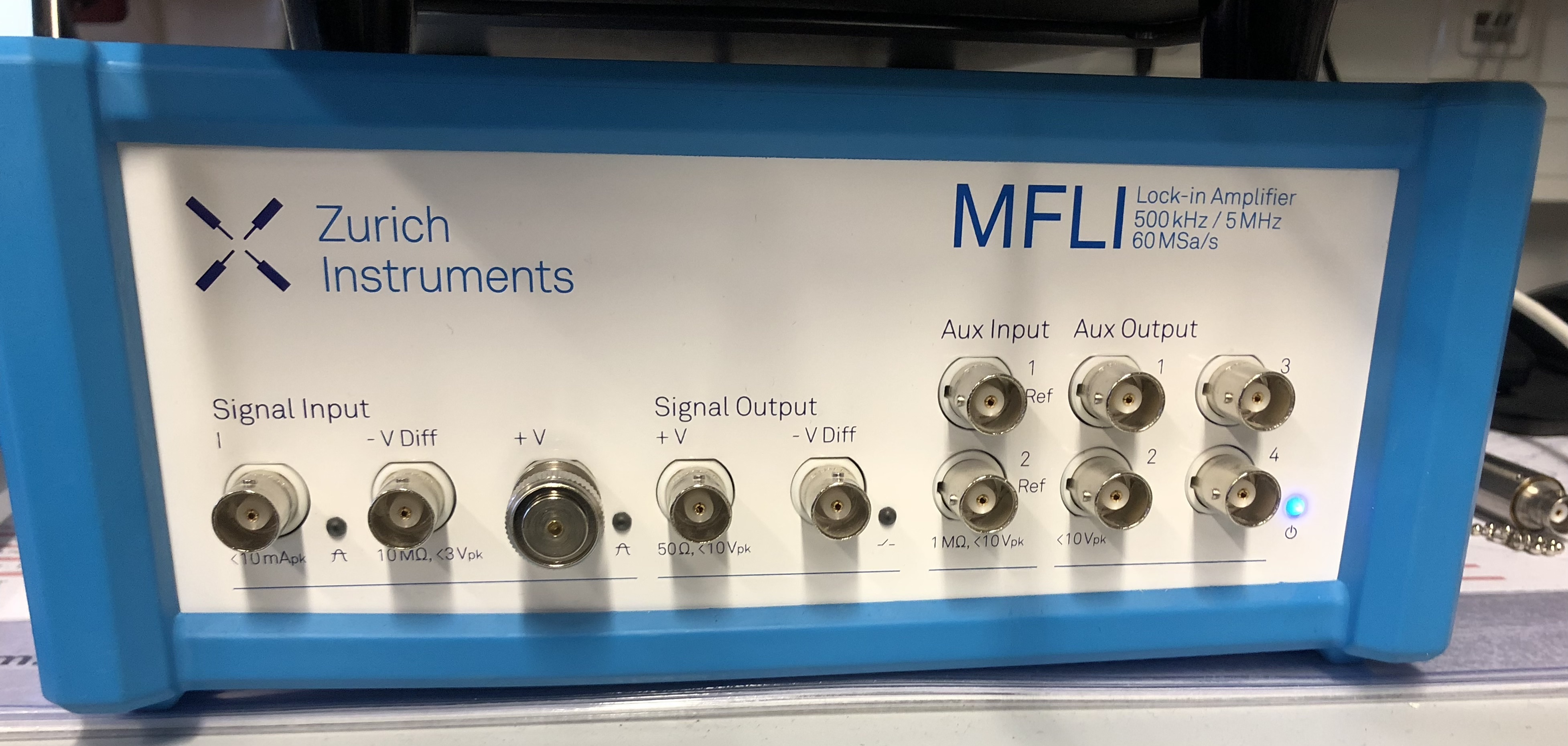
- Zurich Instruments MFLI
- Basel Precision Instruments SP983c
- Stanford Research Systems SR560
- Rigol DSG815 RF source (cabinet below the wet bench in Himmel)
- 4K dipstick with micro-D connector and matching connector with passive elements soldered in
- Low-noise BNC cables
- SMA-BNC adapter
- <details><summary>BNC-to-Banana adapter</summary><img src="https://iffmd.fz-juelich.de/uploads/upload_b692835bdb8fe9a9e4f0a88a11ebd60e.jpg" height="300"/></details>
- <details><summary>Wall socket grounding plug</summary><img src="https://iffmd.fz-juelich.de/uploads/upload_9270538caa83efb175172ff2fe3e867c.jpg" alt="socket grounding plug" height="300"/></details>
- <details><summary>BNC T-piece</summary><img src="https://iffmd.fz-juelich.de/uploads/upload_8558aa19e87aa9c91dec60b4ef2c67fa.png" alt="bnc T-piece" height="300"/></details>
- <details><summary>DUI differential box</summary><img src="https://iffmd.fz-juelich.de/uploads/upload_e2d5ad9a7d854858b8dfe22913efad69.jpg" alt="DUI box" height="300"/></details>
:::
:::success
:::spoiler Recommended acquisition parameters
For the following measurements using the DAQ module of the MFLI (rather than the SCOPE module), the following parameters are a good starting point:
- $f_s = 100\,\mathrm{kHz}$
- $\Delta f = 1\,\mathrm{Hz}$
- $f_\mathrm{osc} = 0\,\mathrm{Hz}$
- $n_\mathrm{avg} = 5$
Using the web interface, the following filter parameters provide sufficient anti-aliasing for the sample rate given above:
- $t_c = 3.5\,\mathrm{μs}$
- $n = 3$ (filter order)
Using `qutil`, the default bandwidth setting automatically sets the filter properties.
Set the bandwidth of the different amplifiers to the largest possible value. We limit the bandwidth using the DAQ to prevent aliasing, but want the amplifiers to pass on as much as possible of what they see at their input.
:::
## 0. Setting up
You can use either the web-interface of the MFLI to acquire spectra or the `qutil.measurement.spectrometer` module. In the latter case, you can use the following code to set up the `Spectrometer` object:
:::spoiler `Spectrometer` setup code
```python
from qutil.measurement.spectrometer import daq, Spectrometer
from zhinst import toolkit
def v(voltage, gain_sr560, **_):
return voltage / gain_sr560
def iv(voltage, gain_basel, **_):
return voltage / gain_basel
session = toolkit.Session('localhost')
device = session.connect_device('dev5247', interface='1gbe')
spect = Spectrometer(
*daq.zhinst.MFLI_daq(session, device),
# procfn=v, processed_unit='V', # for voltage preamp
procfn=iv, processed_unit='A', # for current amp
# the DAQ module returns complex data and therefore the spectrum is two-sided
plot_negative_frequencies=False
)
```
:::
If your measurement settings then contain the keyword `gain_basel` or `gain_sr560`, the displayed spectrum will be correctly adjusted for the level present before the input of the Basel amplifier or SR560 preamplifier, respectively.
:::warning
:::spoiler Data scaling
If you have set a scale in the web interface, the data returned by the device when queried from Python will also be scaled accordingly. Therefore, one must be careful to avoid scaling the data twice (once in the web-interface control and once using a `procfn`).
:::
## 1. Voltage measurements with a mock sample in a 4K dipstick
### 1.1 Setup
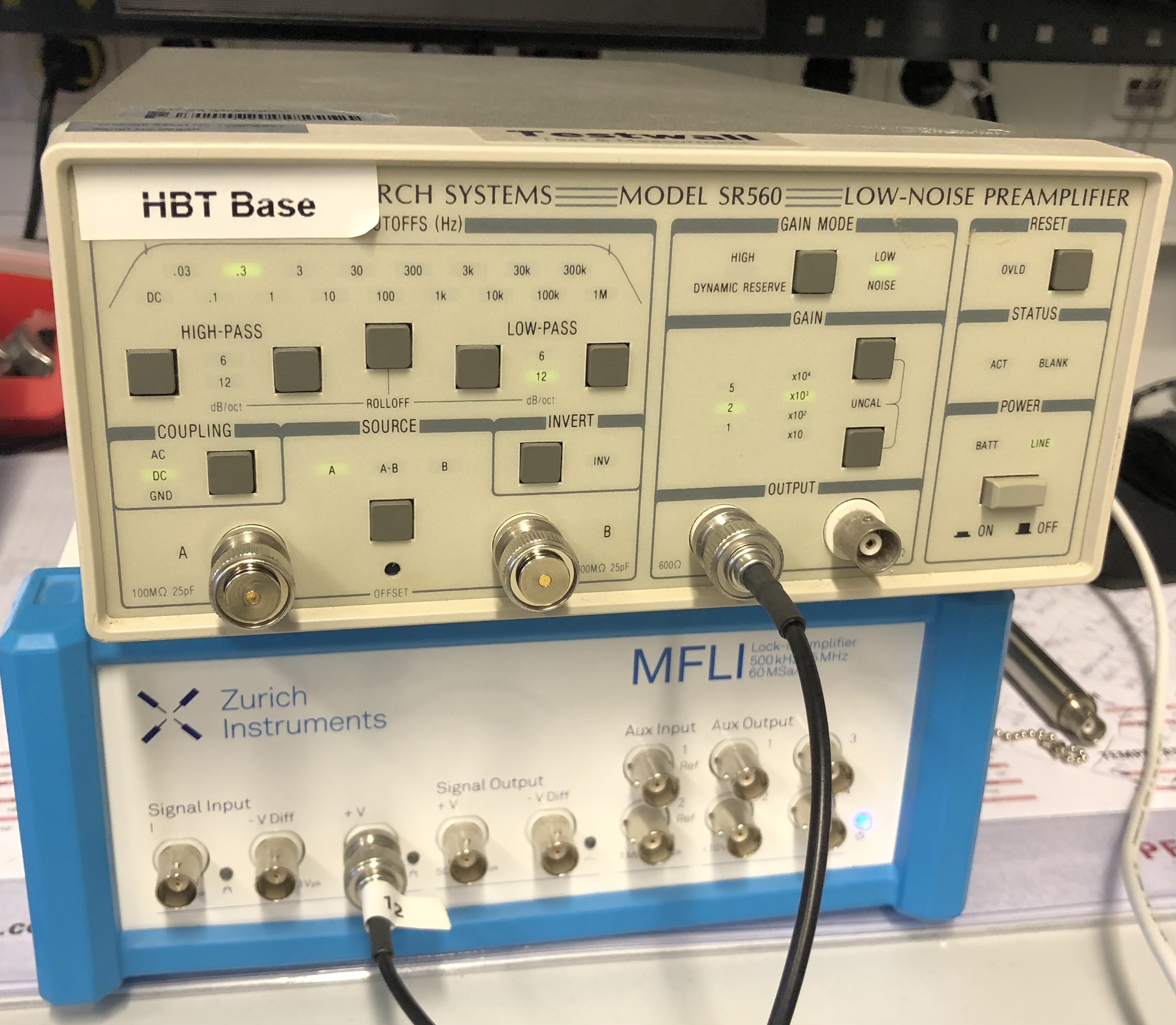
- Set up a Standford Research SR560 preamplifier and connect its output to the voltage input of the MFLI.
- Set the gain of the preamplifier such that the bare noise floor is optimal (according to specs).
### 1.2 Measurement
:::info
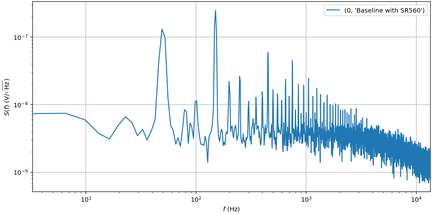
:::spoiler Reference data
Reference data these measurements can be found at `\\janeway\User AG Bluhm\Common\GaAs\Hangleiter\research_techniques\data`. They can be loaded and inspected using `qutil` with (assuming [the setup code](#0-Setting-up) was already executed)
```python
from pathlib import Path
data_path = Path('//janeway/User AG Bluhm/Common/GaAs/Hangleiter',
'research_techniques/data')
spect = Spectrometer.recall_from_disk(data_path / 'spect_sr560_dipstick')
```
:::
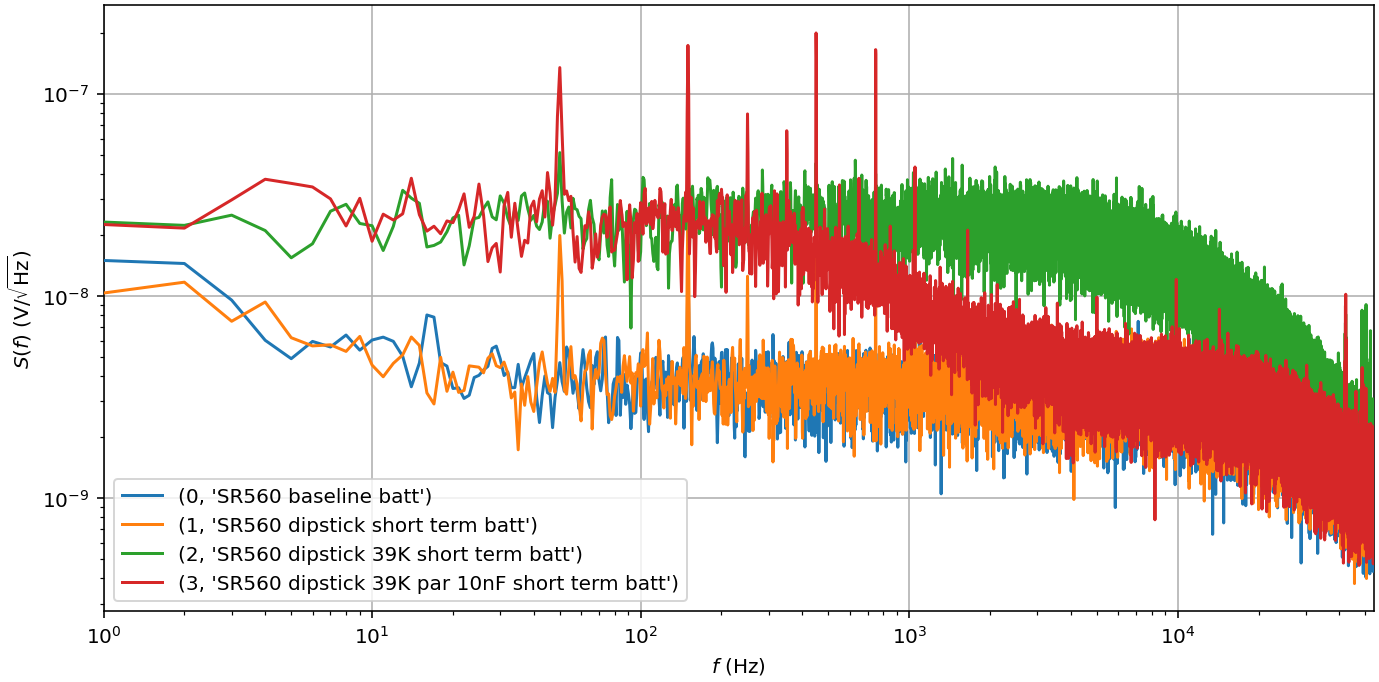
- Connect the voltage input to port 7 of the breakout box and set it to open while setting port 23 to ground.
- What happens to the noise floor? What can you deduce from this about the passive element connected to the open line at the bottom of the dipstick?
:::spoiler Answer
There is a 39 kΩ resistor soldered to the micro-D. This resistor generates thermal (white) noise of $\sqrt{\overline{v_n^2}} = 0.13\sqrt{R}\,\mathrm{nV}/\sqrt{\mathrm{Hz}}\approx 25\,\mathrm{nV}/\sqrt{\mathrm{Hz}}$.
:::
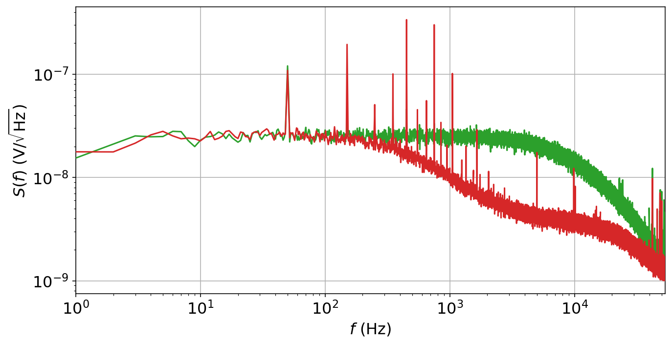
- Plug a T-piece to port 7 and connect the amplifier to one end. Connect the other end to port 24 and open it.
- Can you deduce from the spectrum
- a) what kind of passive element is connected to line 24 and
- b) the magnitude of it?
:::spoiler Answer
There is a 10 nF capacitor soldered to the micro-D. By shorting lines 24 and 7, we connected the capacitor and the resistor (our mock sample) in parallel, thus forming a low-pass RC circuit. The spectrum cuts off at around 500 Hz, giving us a time-constant of ≈2 ms/(2π). Hence, we can estimate the capacitance to be C = τ/R ≈ 8 nF.
:::
:::spoiler Extended `qutil` solution
Clearly, higher frequencies are attenuated, implying we have loaded the amplifier with a low-pass filter. The roll-off of the spectrum would tell us the order of the filter (an $n$-th order RC filter has a roll-off of 20 dB/dec[^zi]). Since we know there is one passive element added to the circuit, it has to be a first-order filter.
Now, assuming there exists a `Spectrometer` object called `spect`, we can display the data in dB, using the spectrum with just the resistor as reference (recall that for power $\mathrm{dB} = 20\log_{10}(V/V_\mathrm{ref})$):
```python
spect.plot_dB_scale = True
spect.plot_amplitude = False # plot power
spect.plot_density = False # plot spectrum
spect.set_reference_spectrum('SR560 dipstick 39K short term batt')
```
We can then read off the frequency at which the spectrum dropped offto 3 dB relative to the one with only the resistor:
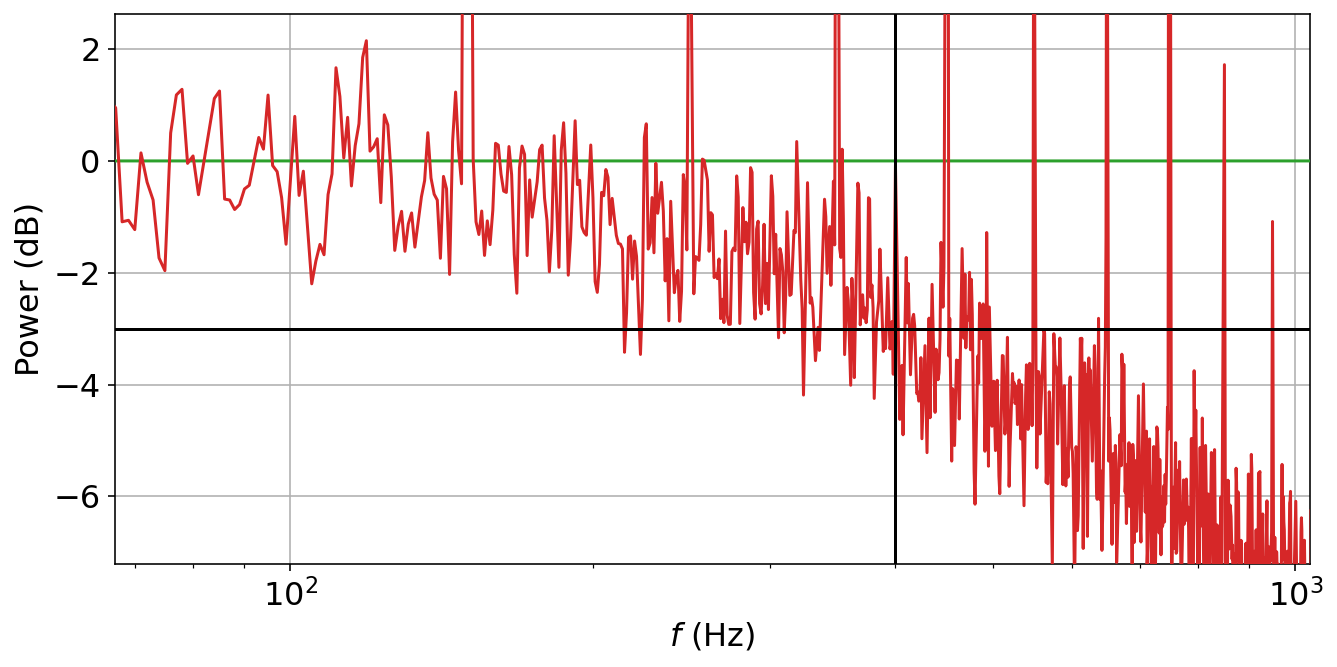
Reading off $f_{3\,\mathrm{dB}} = 400\,\mathrm{Hz}$, we calculate $C = \tau/R = 1/(2\pi f_{3\,\mathrm{dB}} R) = 10.2\,\mathrm{nF}$, which is pretty close to the nominal value of 10 nF.
:::
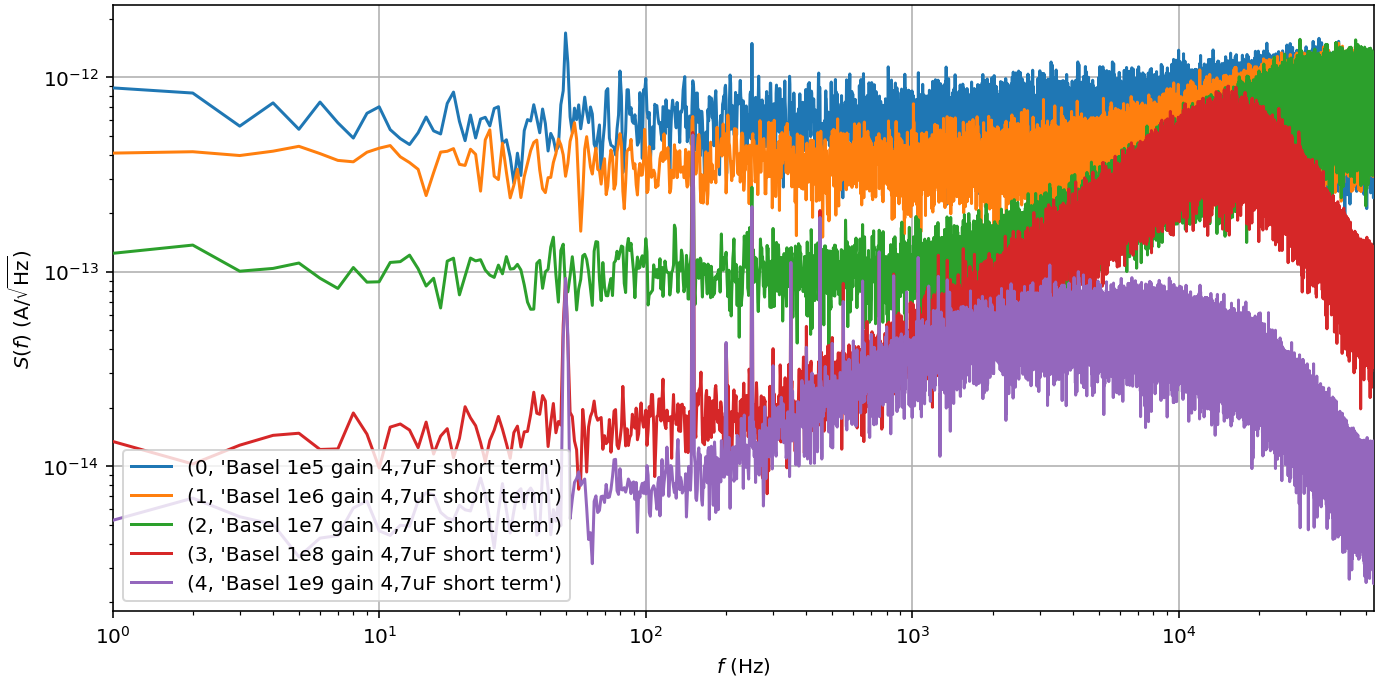
## 2. Current measurements with in-line low-pass filters
### 2.1 Setup
- Set up a Basel amplifier and connect its output to the voltage input of the MFLI. Short the offset voltage input.
- Set the gain of the Basel amplifier to 10^5^ and the bandwidth to full (1 MHz).
- Set up your measurements so that the bare noise floor with the Basel amplifier is optimal (according to specs).
- Connect the current input to ports 20 or 24 of the breakout box and set it to open while setting the other to ground.
### 2.2 Measurement
:::info
:::spoiler Reference data
Reference data these measurements can be found at `\\janeway\User AG Bluhm\Common\GaAs\Hangleiter\research_techniques\data`. They can be loaded and inspected using `qutil` with (assuming [the setup code](#0-Setting-up) was already executed)
```python
from pathlib import Path
data_path = Path('//janeway/User AG Bluhm/Common/GaAs/Hangleiter',
'research_techniques/data')
spect = Spectrometer.recall_from_disk(data_path / 'spect_basel_dipstick')
```
:::
- Measure the noise spectrum at the MFLI for different gains, taking care to stay within the range of the voltage input but staying above their different inherent noise floors.
- Why does the noise floor rise at high frequencies?
:::spoiler Quick answer (longer answer below)
The input load and the feedback resistor of the TIA form a voltage divider for the voltage input noise of the amplifier with transfer function $1 + i\omega R_fC_\mathrm{in}$.
:::
- Why could this be a problem for quantum dot transport measurements?
:::spoiler Answer
Depending on the measurement bandwidth, the filter cutoff can be higher than the rise in voltage noise, leading to "noise-peaking".
:::
:::spoiler Detailed explanation of output voltage noise specs
The output voltage noise is given by the sum of current input noise (converted to voltage by the TIA) and the voltage input noise proliferated by the voltage divider between input impedance and feedback resistor. The current input noise depends only on the magnitude of the feedback resistor $R_f$ (equal to the gain $G$ here) and the Johnson noise it produces,
$$
S_{I,\mathrm{in}}(f; R_f)\approx O(1)\times\sqrt{4k_\mathrm{B}TR_f}.
$$
The voltage input noise of the internal JFETs proliferates to the output multiplied with the voltage division of input impedance $Z_\mathrm{in}(f)$ and feedback resistor $R_f$ as
$$
S_{V,\mathrm{in}}(f; Z_\mathrm{in}, R_f) = S_{V,\mathrm{JFET}}(f)\left(\frac{Z_\mathrm{in}(f) + R_f}{Z_\mathrm{in}(f)}\right),
$$
where the noise profile of the JFETs is typically $1/f$-like.
<details><summary><i>Voltage noise model diagram from the amplifier manual</i></summary><img alt="Basel SP 983c noise gain" src="https://iffmd.fz-juelich.de/uploads/upload_dd99d03ba9e469127c08c52ed0e1df25.png" width="500" /></details>
Hence, in total we have a voltage noise at the output of
$$
S_{V,\mathrm{out}}(f; Z_\mathrm{in}, R_f) = \mathrm{O(1)}\times\sqrt{4k_\mathrm{B}TR_f} + \frac{O(5)}{f}\times\frac{Z_\mathrm{in}(f) + R_f}{Z_\mathrm{in}(f)}
$$
The input impedance is given by a DC resistance of $R_\mathrm{prot}\approx 33\,\Omega$ and an AC component due to the virtual input impedance of the I/V converter, $R_\mathrm{IV}\approx f\times\frac{R_f}{\mathrm{GBWP}}$, with $\mathrm{GBWP}\approx 600\,\mathrm{MHz}$ the gain-bandwidth-product.
<details><summary><i>Input impedance model diagram from the amplifier manual</i></summary><img alt="Basel SP 983c noise gain" src="https://iffmd.fz-juelich.de/uploads/upload_b3ee9d55974dd7612dc33fd46139e3ad.png" width="400" /></details>
For our measurement, the input resistance is in series with a capacitor of about 11 nF, so that, finally, in total we expect our output noise model to follow
$$
S_{V,\mathrm{out}}(f; Z_\mathrm{in}, R_f) = \mathrm{O(1)}\times\sqrt{4k_\mathrm{B}T R_f} + \frac{O(5)}{f}\times\left(1 + \frac{R_f}{\frac{1}{2\pi i f C} + R_\mathrm{prot} + \frac{f R_f}{\mathrm{GBWP}}}\right).
$$
If we measure the output noise for different gains with the input loaded by a 4.7 nF capacitor, we can compare our model to the results:
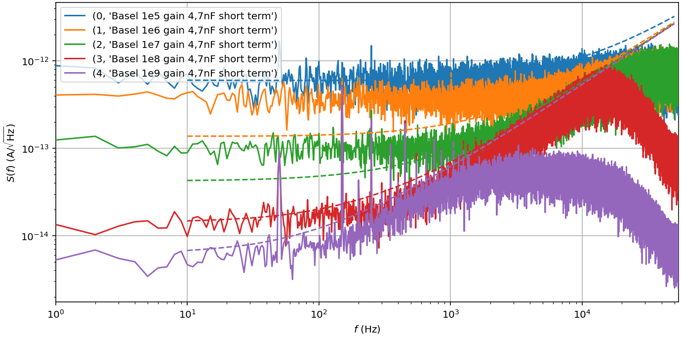
The cutoff towards higher frequencies originates in the finite bandwidth of the lock-in demodulator to prevent aliasing and/or the bandwidth of the Basel amplifier.
:::
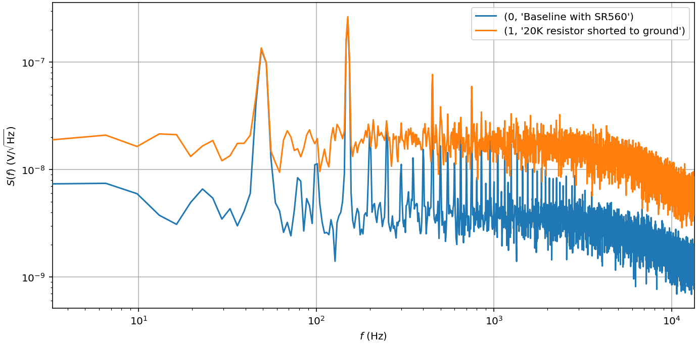
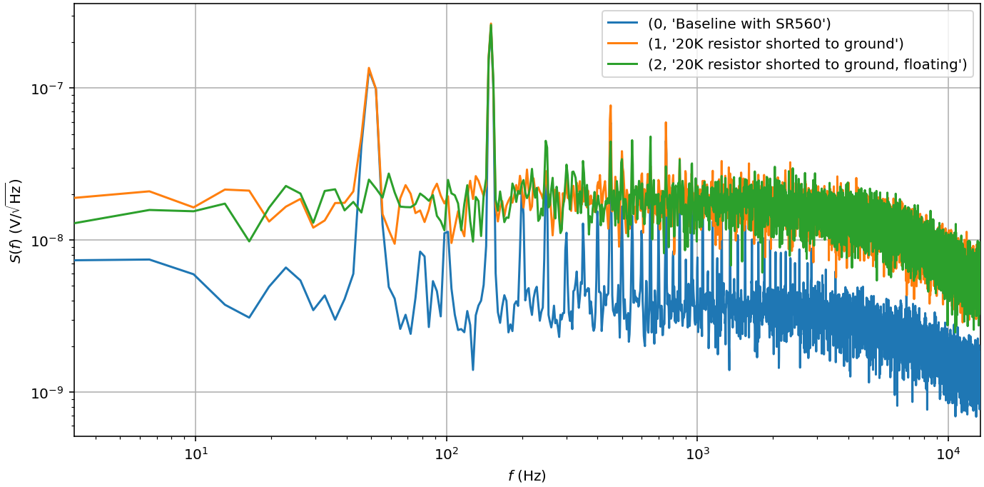
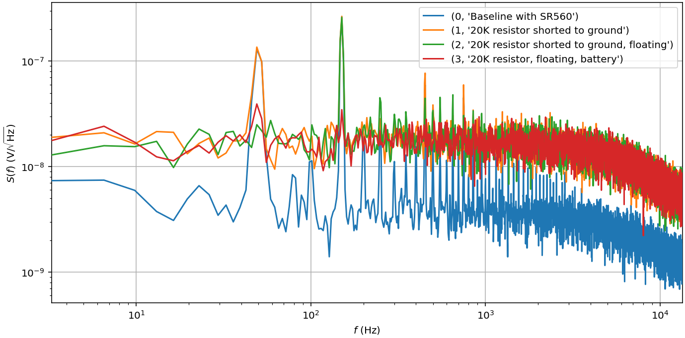
## 3. Grounding
:::info
:::spoiler Reference data
Reference data these measurements can be found at `\\janeway\User AG Bluhm\Common\GaAs\Hangleiter\research_techniques\data`. They can be loaded and inspected using `qutil` with (assuming [the setup code](#0-Setting-up) was already executed)
```python
from pathlib import Path
data_path = Path('//janeway/User AG Bluhm/Common/GaAs/Hangleiter',
'research_techniques/data')
spect = Spectrometer.recall_from_disk(data_path / 'spect_grounding_dipstick')
```
:::
Finally, we will take a look at grounding a (somewhat) complete experimental setup. We will assume that we measure voltages using the SR560, but similar arguments will apply to measuring currents -- the qualitative behavior of course being different as we saw in the previous sections.
The main objective here is to avoid ground loops, i.e., circular connections of the ground conductor with non-zero impedance. These can pick up time-dependent magnetic fields which induce a voltage in the loop.
### 3.1 Setup
Wire the setup for voltage amplification like in [section 1](#1-Voltage-measurements-with-a-mock-sample-in-a-4K-dipstick), loading the (battery-powered) amplifier input with the 39 kΩ resistor (lines 7 or 23) shorted to ground and establish a noise baseline.
In practice, DAQ devices are often connected to the computer controlling the experiment, for instance via PCIe, and are thereby grounded through the computer chassis. Hence, their ground connections are not easily broken, and in order to avoid ground loops, one needs to insert a ground breaker earlier in the signal chain.
While in principle, the MFLI allows floating its input, we will not make use of it here in order to emulate measuring using, for instance, an Alazar digitizer card (although you're welcome to test out the effect of a floating input of course!)
### 3.2 Measurements
In typical experiments, high-frequency signals such as AWG pulses or microwave bursts need to be applied to the sample. Since the coaxial cables carrying these need to have good ground connections in order to avoid impedance mismatches, breaking the ground connection of RF instruments is typically disadvantageous. Hence, we use them to supply the ground to the cryostat in the first place.
Here, we will use a Rigol RF source as exemplary instrument.
- To start off, plug the Rigol into a different wall outlet and connect the LF output to SMA port 2 of the dipstick. What changes?
:::spoiler Answer
Since the Rigol and the MFLI are plugged into different outlets and share a ground connection via the dipstick, we introduced a large ground loop that picks up stray signals.
:::
- Plug the Rigol instead into the same outlet as the MFLI. Again acquire a spectrum.
- Turn on the Rigol. Does something change in the noise spectrum?
:::spoiler Answer
Certain instruments have soft power switches and introduce noise even when nominally off.
:::
- Terminate the coaxial cable in the dipstick with a 50 Ω connector. Program the Rigol to output a 9.8 kHz sine wave with an amplitude of 100 mV at the LF port. Acquire a spectrum. Why do you see the tone in the noise spectrum?
:::spoiler Answer
The RF signal sends a current to ground through the 50 Ω load impedance, which gets picked up by the spectrometer through the resistive load at its input.
:::
- Now insert the DIY differential box into the signal path. Connect the input to the output of the SR560 and the two outputs to the V+ and V- inputs of the MFLI. Switch the MFLI to differential input and acquire a noise spectrum. Why does the forest of high-frequency interference peaks disappear?
:::spoiler
We break the ground loop by subtracting the signals on the inner and outer conductors of the coaxial cable.
In case the DAQ of choice does not offer a differential input, one can also use a unity-gain buffer such as an [AMP03](https://www.analog.com/media/en/technical-documentation/data-sheets/amp03.pdf) instead. However, here one needs to take care not to introduce another ground loop through the power supply of the AMP03 and should power it either using a battery or by isolating the grounds of the amplifier and the power supply.
Note that while the bandwidth of the AMP03 is limited, that of the DIY box is not.
:::
*[TIA]: Trans-Impedance Amplifier
*[JFETs]: Junction-gate Field-Effect Transistors
*[DAQ]: data acquisition
*[DUT]: device-under-test
*[DAC]: digital-to-analog
*[ADC]: analog-to-digital
*[DIY]: do-it-yourself
[^zi]: https://www.zhinst.com/europe/en/resources/principles-of-lock-in-detection
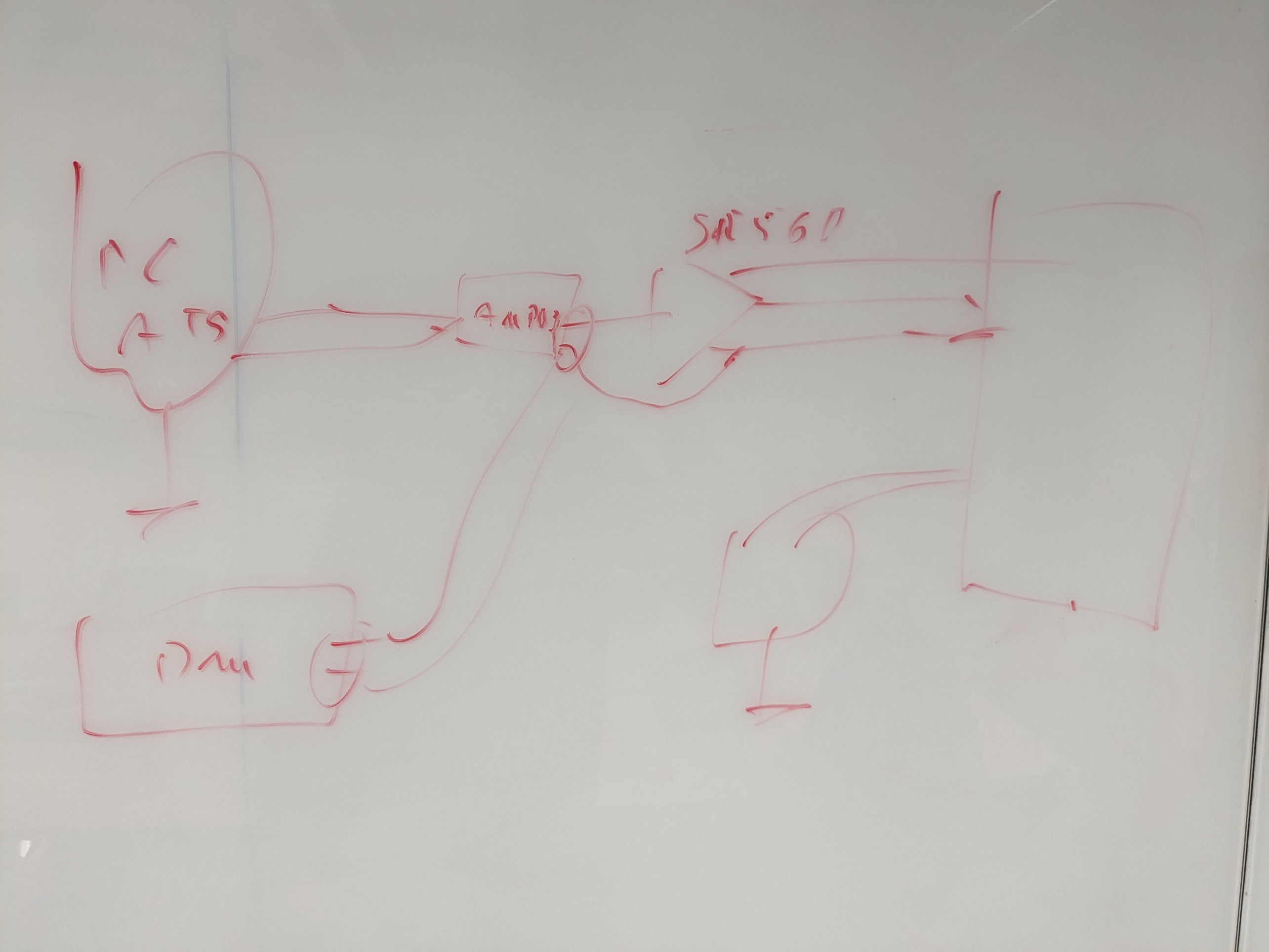
<!--
20-24: 11 nF
07-23: 39 K
notes
------
- start with clean setup
- dipstick, 39K, SR560 (battery), MFLI
- connect rigol LF to SMA 2 of dipstick
- do not turn on yet
- turn Rigol on
- Connect 50R cap to RF line 2 at bottom
- Set LF output Rigol to
- 9.8 kHz
- 100 mV amplitude
- sine
- connect DIY box
- set mfli to differential input
- monitor 9.8 kHz peak
-------------------------------------------
# Material dump
-------------------------------------------
## Aliasing
- [ ] Place grounding cap on MFLI +V input
- [ ] Download [mfli config file](https://moodle.rwth-aachen.de/pluginfile.php/2453685/mod_folder/content/0/research_techniques.xml?forcedownload=1) and apply it in on the device config tab
- [ ] Run the spectrum tab
## Amplifier noise
- [ ] Connect 50Ω output of SR560 preamplifier to the +V input of the MFLI as in photo below
- [ ] Load config and run Spectrum tab
- [ ] Set gain on preamp to 1. Why is the [specified noise figure](https://www.thinksrs.com/downloads/pdfs/catalog/SR560c.pdf) of 4nV/sqrt(Hz) not reached?
<details><summary>Short explanation</summary>
Best preamp performance only availible at sufficient gain. For gain 100 a noise figure of 3.2 nV/sqrt(Hz) was measured
</details>
## Breakout-Box ground connection
1 Ohm Breakoutbox with bad GND
40 mOhm Breakoutbox Fischer over 2m cable
30 mOhm Breakoutbox Fischer to Fischer connection
20 mOhm Breakoutbox Fischer to Fischer with additional GND harness
## Clipping
:::spoiler image dump
:::
-->